Simplified Time-Series Analytics Using the time_bucket() Function
If you are working with time-series data, you need a way to be able to easily manipulate, query, and visualize that data. Often times, time-series databases contain a number of time-oriented functions that aren't found in traditional databases.
These functions are meant to provide two key benefits: improved ease of use for time-series analytics, and improved performance. In this case, I'm going to demonstrate with two TimescaleDB functions time_bucket()and time_bucket_gapfill().
The functions live alongside full SQL and can be viewed as extensions of the SQL language. Since a vast amount of developers today already know SQL, the learning curve is greatly reduced. Time_bucket() is used for aggregating arbitrarily-sized time periods and gapfill() is important when your time buckets have missing data or gaps, which is a very common occurrence when capturing 1000s of time series readings per second.
In this blog, I'll discuss both of these capabilities and show them in action using Grafana.
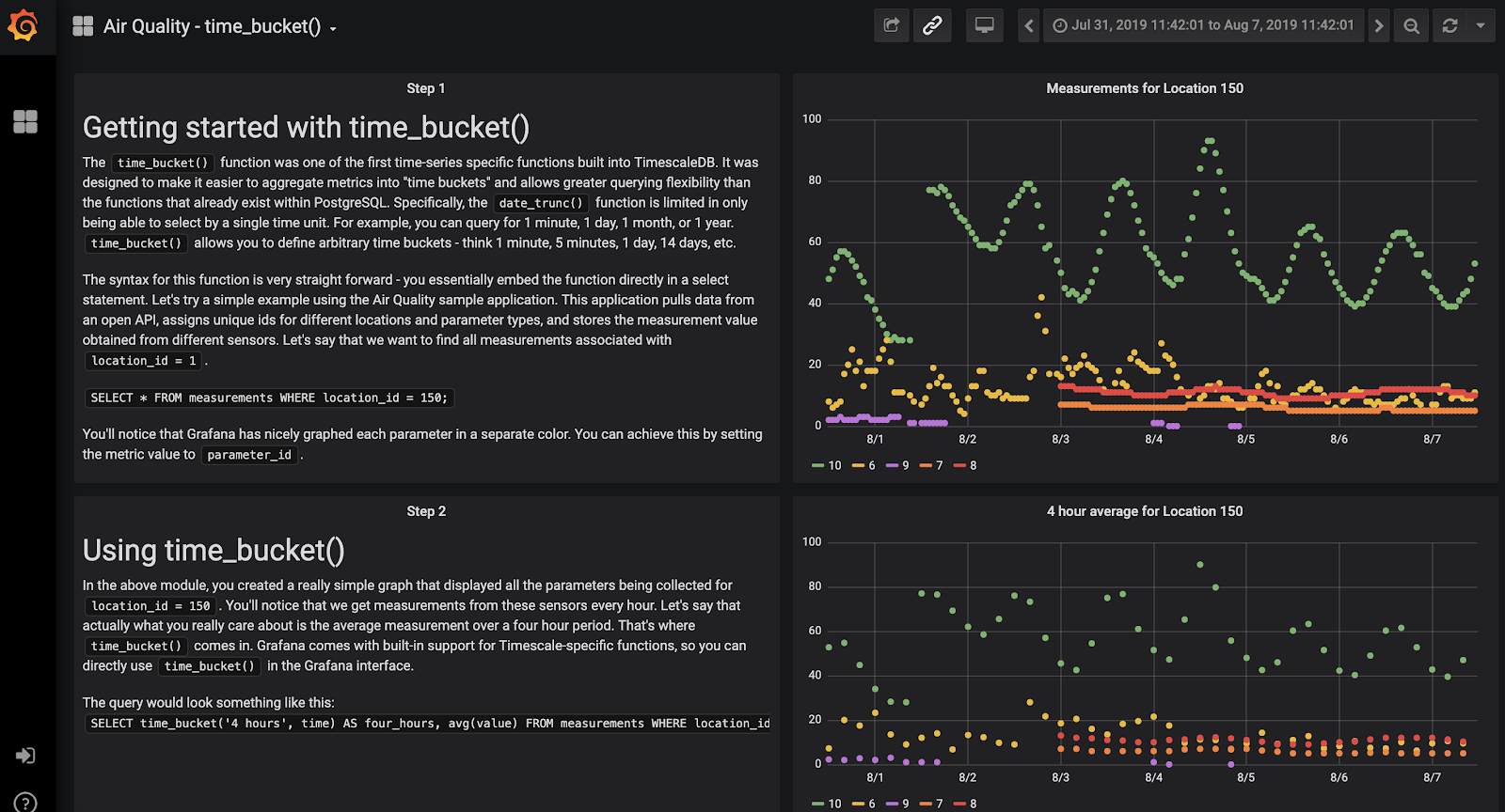
Check out this Grafana dashboard that is visualizing data from TimescaleDB (both hosted in Timescale Cloud) showing time bucketing and gapfilling in action.

Background on time_bucket()
Essentially, time_bucket() is a more powerful version of the standard PostgreSQL date_trunc()function. date_trunc “truncates” a TIMESTAMP or an INTERVAL value based on a specified date part (e.g. hour, week or month) and returns the truncated timestamp or interval.
For example, date_trunc can aggregate by 1 second, 1 hour, 1 day or 1 week. However, users often want to see aggregates by 5 minutes or 4 hours, etc. This can get pretty complicated in SQL, but time_bucket() makes it easy.
Time bucketing allows for arbitrary time intervals (e.g., 5 minutes, 6 hours, etc.), as well as flexible groupings and offsets, instead of just second, minute, hour, and so on.
In addition to allowing more flexible time-series queries, time_bucket() also allows you to write these queries in a simpler way. In fact, it knows to infer the time range directly from the WHERE clause, which greatly simplifies the query syntax.
Here it is in action:
SELECT time_bucket('5 minutes', time) AS five_min, avg(cpu)
  FROM metrics
  GROUP BY five_min
  ORDER BY five_min DESC LIMIT 12;
When to use time_bucket()
As you can imagine, time bucketing can be helpful for a number of scenarios. When it comes to creating dashboards or visualizations of time-series data, many rely on this function to turn their raw observations into fixed time intervals.
When graphing time-series data using a solution such as Grafana, aggregations can help identify trends over time by grouping raw data into higher-level aggregates. For example, you might want to average monthly raw data daily to achieve a smoother trend line or count the number of occurrences of non-numeric data.
Building on top of time_bucket() with time_bucket_gapfill()
One issue users often encounter when working with time-series data is recording measurements at irregular or mismatched intervals. This creates a time bucket interval with missing data or gaps. Fortunately, TimescaleDB has a function called time_bucket_gapfill() that allows you to aggregate your data into continuous time intervals. You can choose two different ways to fill in gaps: locf()which carries the last known value in the time range forward or interpolate() which does a linear interpolation between gaps.
Get hands-on with a sample application
Now that you know what time_bucket() and time_bucket_gapfill() do, it’s time to get hands-on with a sample application! I’ve built a simple Python application that pulls data from the Open AQ Platform API (an open API air quality data). Essentially, the application reads the API to get air quality values for all cities in Great Britain over period of time, parses the results, and stores all measurements collected from air quality sensors in TimescaleDB.
All the code for this application can be found on GitHub.
I also connected a Grafana instance to the TimescaleDB database that stores these results and have written a step-by-step tutorial of how to use time_bucket() and time_bucket_gapfill() to visualize the data.
Feel free to explore my Grafana dashboard or build your own!

