Building a Regression Model Using Oracle Data Mining
In this article, I will do regression analysis with Oracle data mining.

Data science and machine learning are very popular today. But these subjects require extensive knowledge and application expertise. We can solve these problems with various products and software that have been developed by various companies. In Oracle, methods and algorithms for solving these problems are presented to users with the DBMS_DATA_MINING package.
With the DBMS_DATA_MINING package, we can create models such as clustering, classification, regression, anomaly detection, feature extraction, and association. We can interpret efficiency with the models we create. The results we obtain from these models can be put into our business scenario.
The DBMS_DATA_MINING package does not come up by default on the Oracle database. For this reason, it's necessary to install this package first. You can set up your database with Oracle data mining by following this link.
With the installation of the Oracle data mining package, three new dictionary tables are created:
SELECT * FROM  ALL_MINING_MODELS;
SELECT * FROM ALL_MINING_MODEL_SETTINGS;
SELECT * FROM ALL_MINING_MODEL_ATTRIBUTES;
The ALL_MINING_MODELS table contains information about all the models.

The ALL_MINING_MODELS_SETTINGS and ALL_MINING_MODELS_ATTRIBUTES tables contain parameters and specific details about these models.
Now, let's prepare an easily understood data set to do market basket analysis.
We need a dataset to do the example. We will do this example through the BOSTON_HOUSING dataset we downloaded from kaggle.
Let's first examine the BOSTON_HOUSING dataset.
| Column Name | Description | Data Type |
| crim | per capita crime rate by town. | Number |
| zn | proportion of residential land zoned for lots over 25,000 sq.ft. | Number |
| indus | proportion of non-retail business acres per town. | Number |
| chas | Charles River dummy variable (= 1 if tract bounds river; 0 otherwise). | Number |
| nox | nitrogen oxides concentration (parts per 10 million). | Number |
| rm | average number of rooms per dwelling. | Number |
| age | proportion of owner-occupied units built prior to 1940. | Number |
| dis | weighted mean of distances to five Boston employment centres. | Number |
| rad | index of accessibility to radial highways. | Number |
| tax | full-value property-tax rate per $10,000. | Number |
| ptratio | pupil-teacher ratio by town. | Number |
| black | 1000(Bk – 0.63)^2 where Bk is the proportion of blacks by town. | Number |
| lstat | lower status of the population (percent). | Number |
| medv | median value of owner-occupied homes in $1000s. | Number |
Now that we have reviewed the details with our dataset, let's load the BOSTON_HOUSING that we downloaded to our Oracle database.
First, create the Oracle table in which we will load the data set (train.csv) that we downloaded.
CREATE TABLE BOSTON_HOUSING
(
   ID        NUMBER,
   CRIM      NUMBER,
   ZN        NUMBER,
   INDUS     NUMBER,
   CHAS      NUMBER,
   NOX       NUMBER,
   RM        NUMBER,
   AGE       NUMBER,
   DIS       NUMBER,
   RAD       NUMBER,
   TAX       NUMBER,
   PTRATIO   NUMBER,
   BLACK     NUMBER,
   LSTAT     NUMBER,
   MEDV      NUMBER
);
Now that we have created our table, we will load the dataset we downloaded as CSV into the table; we have multiple methods to do this:
Using Oracle External Table
Using Oracle SQL Loader
Using SQL-PL/SQL editors (Oracle SQL Developer, Toad, PL/SQL Developer, etc.)
I will load the dataset with the editor that I am using. I use Toad as an editor. With Toad, you can perform the data loading process by following the steps below.
Database > Import > Import Table Data
You may not be using this editor because Toad is paid. This feature is available to other editors, so you can easily do this with other editors. For example, with Oracle SQL Developer for free, you can load data as follows using Oracle SQL Developer.
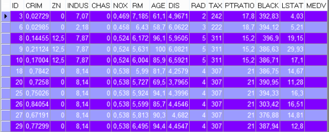
SELECT * FROM BOSTON_HOUSING; We have completed the dataset installation process.
When we observe the data, we see the details according to the various characteristics of the houses. Each row contains information on the specific characteristics of the house. Our basic parameters for regression analysis are as presented in this table. In this table, we predict the result of regression analysis. The MEDV column is the target variable that we will use in this analysis.
Before starting the regression analysis, I will give some information about the algorithm used to better understand the subject.
The DBMS_DATA_MINING package is implemented by the Generalized Linear Model algorithm. To use this algorithm, we need to define some parameters. These parameters are as follows:
 Now let's create the table where we will read the algorithm settings.
CREATE TABLE SETTINGS_GLM
AS
SELECT *
     FROM TABLE (DBMS_DATA_MINING.GET_DEFAULT_SETTINGS)
    WHERE SETTING_NAME LIKE '%GLM%';

BEGIN
   INSERT INTO SETTINGS_GLM
        VALUES (DBMS_DATA_MINING.ALGO_NAME, 'ALGO_GENERALIZED_LINEAR_MODEL');

   INSERT INTO SETTINGS_GLM
        VALUES (DBMS_DATA_MINING.PREP_AUTO, 'ON');

   INSERT INTO SETTINGS_GLM
        VALUES (
                  DBMS_DATA_MINING.GLMS_RIDGE_REGRESSION,
                  'GLMS_RIDGE_REG_DISABLE');

   INSERT INTO SETTINGS_GLM
        VALUES (
                  DBMS_DATA_MINING.ODMS_MISSING_VALUE_TREATMENT,
                  'ODMS_MISSING_VALUE_MEAN_MODE');

   COMMIT;
END;
Yes, we created the table to read the algorithm parameters. Now we can go on creating our model.
CREATE OR REPLACE VIEW VW_BOSTON_HOUSING AS SELECT * FROM BOSTON_HOUSING;

BEGIN
   DBMS_DATA_MINING.CREATE_MODEL(
      model_name            => 'MD_GLM_MODEL',
      mining_function       =>  DBMS_DATA_MINING.REGRESSION,
      data_table_name       => 'VW_BOSTON_HOUSING',
      case_id_column_name   => 'ID',
      target_column_name    =>  'MEDV',
      settings_table_name   => 'SETTINGS_GLM');
END;
Our model has occurred, now look at the details of our model from the dictionary.
SELECT MODEL_NAME,
       ALGORITHM,
       COMMENTS,
       CREATION_DATE,
       MINING_FUNCTION,
       MODEL_SIZE
  FROM ALL_MINING_MODELS
 WHERE MODEL_NAME = 'MD_GLM_MODEL';
SELECT SETTING_NAME, SETTING_VALUE
FROM ALL_MINING_MODEL_SETTINGS
WHERE MODEL_NAME = 'MD_GLM_MODEL';
The Anova table of the Regression model we have created can be accessed as follows.
SELECT * FROM
TABLE (DBMS_DATA_MINING.GET_MODEL_DETAILS_GLM ('MD_GLM_MODEL'));
Let's see how we can test with our model now. First of all, we create the table that we need to load the test.csv data that we have downloaded from kaggle and we import the data in it.
CREATE TABLE BOSTON_HOUSING_TEST
(
   ID        NUMBER,
   CRIM      NUMBER,
   ZN        NUMBER,
   INDUS     NUMBER,
   CHAS      NUMBER,
   NOX       NUMBER,
   RM        NUMBER,
   AGE       NUMBER,
   DIS       NUMBER,
   RAD       NUMBER,
   TAX       NUMBER,
   PTRATIO   NUMBER,
   BLACK     NUMBER,
   LSTAT     NUMBER,
   MEDV      NUMBER
);
Database –> Import –> Import Table Data (test.csv)
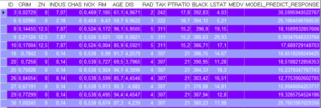
SELECT * FROM BOSTON_HOUSING_TEST; Now run the model that we created with the test data and look at the results.
SELECT T.*,
 PREDICTION (MD_GLM_MODEL USING *) MODEL_PREDICT_RESPONSE
FROM BOSTON_HOUSING_TEST T;

