Predicting Housing Prices Using Google AutoML Tables
Overview of Problem
Tabular data is quite common in various business and engineering problems. Machine learning can be used to predict particular columns of the table we are interested in, using other columns as input features. We will take an example of using historical house sales data to predict sales prices for houses that come on the market in the future. The house prices dataset from Kaggle contains such data for Ames, Iowa. It contains predictive columns like house area, neighborhood area name, type of building, house style, condition, year last sold, etc., among a total of 79 such predictive features. Some of these features are categorical while others are numerical and our goal is to predict the Sale Price (a numeric column) of houses using these features.
|
Id
|
LotArea
|
Neighborhood
|
BldgType
|
Style
|
Cond
|
YrBuilt
|
1stFlrSF
|
2ndFlrSF
|
Fireplaces
|
YrSold
|
SalePrice
|
| 1 |
8450
|
CollgCr
|
1Fam
|
2Story
|
5 |
2003
|
856
|
854
|
0 |
2008
|
208500
|
| 2 |
9600
|
Veenker
|
1Fam
|
1Story
|
8 |
1976
|
1262
|
0 | 1 |
2007
|
181500
|
| 3 |
11250
|
CollgCr
|
1Fam |
2Story
|
5 |
2001
|
920
|
866
|
1 |
2008
|
223500
|
| 4 |
9550
|
CollgCr
|
1Fam
|
2Story
|
5 |
1915
|
961
|
756
|
1 |
2006
|
140000
|
| 5 |
14260
|
NoRidge
|
1Fam
|
2Story
|
5 |
2000
|
1145
|
1053
|
1 |
2008
|
250000
|
| 6 |
14115
|
Mitchel
|
1Fam
|
1.5Fin
|
5 |
1993
|
796
|
566
|
0 |
2009
|
143000
|
| 7 |
10084
|
Somerst
|
1Fam
|
1Story
|
5 |
2004
|
1694
|
0 | 1 |
2007
|
307000
|
| 8 |
10382
|
NWAmes
|
1Fam
|
2Story
|
6 |
1973
|
1107
|
983
|
2 |
2009
|
200000
|
| 9 |
6120
|
OldTown
|
1Fam
|
1.5Fin
|
5 |
1931
|
1022
|
752
|
2 |
2008
|
129900
|
| 10 |
7420
|
BrkSide
|
2fmCon
|
1.5Fin
|
6 |
1939
|
1077
|
0 | 2 |
2008
|
118000
|
| 11 |
11200
|
Sawyer
|
1Fam
|
1Story
|
5 |
1965
|
1040
|
0 | 0 |
2008
|
129500
|
| 12 |
11924
|
NridgHt
|
1Fam |
2Story
|
5 |
2005
|
1182
|
1142
|
2 | 2006 |
345000
|
| 13 |
12968
|
Sawyer
|
1Fam
|
1Story
|
6 |
1962
|
912
|
0 | 0 |
2008
|
144000
|
Overview of Google AutoML Tables
Google AutoML Tables enables quick and high accuracy training and subsequent hosting of ML models for such a problem. Users can import and visualize the data, train a model, evaluate it on a test set, iterate on improving model accuracy and then host the best model for online/offline predictions. All of the above functionality is available as a service without any ML expertise or hardware or software installation required from users.
AutoML table can train both regression and classification models depending on the type of column we are trying to predict.
Initial Setup
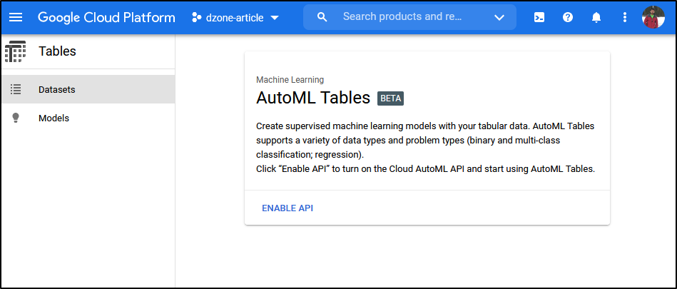
We first log in to our Google Cloud Platform (GCP) account (or create it if we don't have one) and create a new project. Then enable AutoML Tables by selecting 'Tables' and enabling the API as shown below.


Importing Data
To import data, we go to the Import tab and select the source type, i.e., either CSV or BigQuery table. In our case, we will upload the 'train.csv' of the housing prices dataset that we downloaded earlier. If an upload destination GCS bucket doesn't already exist, we can create a single region bucket, e.g., 'gs://house_prices_dataset_1'. AutoML Tables will import the data and auto analyze it to validate it and detect the datatypes of columns.
Exploring Data
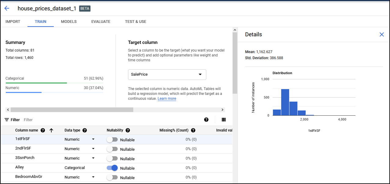
We can explore the imported data schema once import completes. AutoML will show the column names, data type (i.e., category, numeric, or text), missing values, and distinct values for each column. We should set the prediction target column and in our case, we'll predict the SalePrice column. To enable us to understand how valuable each feature is individually, it also generates correlation scores of each column with the target column. In addition, we can explore the distribution of values in each column.
In some cases, it's possible that feature datatype is incorrectly detected as numeric when it is actually categorical if the category values are numeric instead of text, for example, Year Sold. We can override the type in case of such mistakes.
We can now select the input columns and certain data and training parameters. We first remove the ID column as a feature, since it's a unique identifier of the row and not a feature. We then specify the train, validation, and test dataset split that AutoML will use during training. This can be set to happen either automatically(randomly) or we can specify Train/Validation/Test set rows with an additional column. Next, we can set whether any column should be considered as a weight column. This will give higher importance to certain rows and is helpful if we want our model to be more accurate for certain subsets of data, for example for certain house types or regions.
In advanced features, we can select the duration for which we should train the model. In case the model converges earlier, AutoML will automatically stop training ('Early stopping') before our specified duration. Since our dataset is small, we can select a budget of just 1 hour.
Finally, we can select objective functions from among:
- RMSE (Root Mean Square Error) — This objective function is used when large deviations or small relative deviations on large values should matter more.
- MAE (Mean Absolute Error) — This is similar to RMSE but large deviations matter slightly less since we take the absolute difference (L1) instead of squared difference (L2) as in RMSE.
- RMSLE (Root Mean Square Log Error) — This objective function is used when we want to treat large and small scale deviations equally since we take a log of predictions and ground truth.
Testing and Results
Training the model can take between 30 min to 20 hours depending on the budget specified and convergence of training. Once completed, we can see the results of our regression model where we are able to predict within 14% of the actual price on average (MAPE) on the test split of our training data. With more training data, this error can be further reduced.

We can also see an importance score for each of the features. We see that 'Ground Living Area' is the most important feature. Other top features are 'Lot Area,' 'Open Porch Area,' '1st Floor Area,' 'Quality of House,' 'Year Built,' 'Year Remodelled,' etc., which are quite intuitive and indicate that model is learning the correct features to predict sales price.

Prediction
We can use this model in 3 modes for prediction on new data:
- Online prediction — In online mode, we can issue live requests to our model, e.g., from a production service. The model is hosted by AutoML which will replicate the model and deliver a high-availability and low-latency SLO. For this mode, the model needs to be deployed.
- Batch prediction — In batch mode, the model can be run for one-off jobs by AutoML to predict over a bigger batch of data we already have. There is no need to deploy the model and is thus cheaper than online mode.
- Self-hosted — We can export a docker image of the model and host it on our own VMs and containers. In this mode, we will be responsible for the reliability and maintenance of the model. This mode is useful if the model needs to be used on-prem for predicting data that can not leave an on-prem environment or if the costs of using AutoML online/batch prediction are too high.


Conclusion
To conclude, in this article, we showed how AutoML Tables is a great tool to train and host a good quality ML model for tabular data while requiring only minimal knowledge of ML/AI and no efforts for setting up training and hosting environments.
AutoML Tables take care of these requirements for you and provides you with 'Automatic ML.'


